What is Linda?
Linda is the name of a CrossFit benchmark workout. The original form of the workout is 10-9-8-7-6-5-4-3-2-1 reps of the triplet
- deadlift at 1.5 times bodyweight
- bench press at bodyweight
- clean at 0.75 times bodyweight
Linda was included in the 2018 CrossFit regionals in a standardized form. Based off the average bodyweight of CrossFit games athletes, it was 10-9-8-7-6-5-4-3-2-1 reps of the triplet (weights listed are male/female)
- deadlift at 295/220 lb.
- bench press at 195/135 lb.
- squat clean at 145/105 lb.
Since the weights are fixed, it seems plausible that heavier athletes will finish higher on regionals Linda than lighter athletes. The goal of this post is to make the relationship between bodyweight and Linda finish more precise. To phrase it as a question: if you know an athlete’s bodyweight, how much information does that give you about their Linda finish?
Data Cleaning
I’m using the same data I used for the visualizations of the regionals, placed in a tibble called regionals:
regionals## # A tibble: 4,308 x 13
## rank_overall id age weight height name event rank points time
## <dbl> <dbl> <dbl> <dbl> <dbl> <chr> <dbl> <dbl> <dbl> <dbl>
## 1 1 55121 25 150 66.5 Katr… 1 1 100 2470.
## 2 2 305891 29 139 63 Kari… 1 4 84 2583.
## 3 3 103389 30 140 65.0 Caro… 1 2 94 2532.
## 4 4 3200 30 148 66 Dani… 1 18 44 2752.
## 5 5 236779 26 146 67 Chlo… 1 24 32 2797.
## 6 6 239148 28 143 63 Caro… 1 12 56 2671.
## 7 7 115892 26 150 66 Meg … 1 14 52 2697.
## 8 8 497688 25 160 67 Kate… 1 17 46 2725.
## 9 9 116926 29 152 67.7 Kari… 1 10 60 2645.
## 10 10 255576 33 155 67 Ashl… 1 5 80 2586.
## # ... with 4,298 more rows, and 3 more variables: cumulative_points <dbl>,
## # location <chr>, gender <chr>Let’s look at a summary of the male weights. The weights are self-reported, so there might be some bad data we need to remove. In the process of gathering the data, I converted all weights to pounds (some were originally listed in kilograms).
regionals %>%
  filter(gender == "Male") %>%
  select(name, weight) %>%
  distinct() %>%
  select(weight) %>%
  summary()
## weight
## Min. :115.0
## 1st Qu.:185.0
## Median :194.0
## Mean :192.7
## 3rd Qu.:200.0
## Max. :229.3
## NA's :1The average of 193 lbs is slightly below the average US male weight of 196 lbs. The maximum of about 230 lbs doesn’t sound any alarm bells, but the minimum of 115 lbs is definitely suspicious. After investigating further, this corresponds to an athlete listed as 4 ft. 8 in. in height, which is obviously incorrect, so I will throw out this point. The remaining weights at the lower end seem fine:
regionals %>%
  filter(gender == "Male", weight != 115) %>%
  select(name, weight) %>%
  distinct() %>%
  arrange(weight)
## # A tibble: 358 x 2
## name weight
## <chr> <dbl>
## 1 Josh Workman 155
## 2 Rubén Insua 159.
## 3 Ivan Gaitan 161.
## 4 Uriel Bloch 161.
## 5 Gilson Duarte 162
## 6 Alexander Anasagasti 163.
## 7 Tom Lengyel 165
## 8 Aaron Osborne 165.
## 9 Miguel Garduno 167
## 10 ates boran 169
## # ... with 348 more rowsHere is a histogram of the male weight distribution:
regionals %>%
  filter(gender == "Male", weight != 115, !is.na(weight)) %>%
  select(name, weight) %>%
  distinct() %>%
  ggplot(aes(weight)) +
  geom_histogram(breaks = seq(150, 230, 5), color = "black", fill = "orange") +
  scale_x_continuous(breaks = seq(150, 230, 5))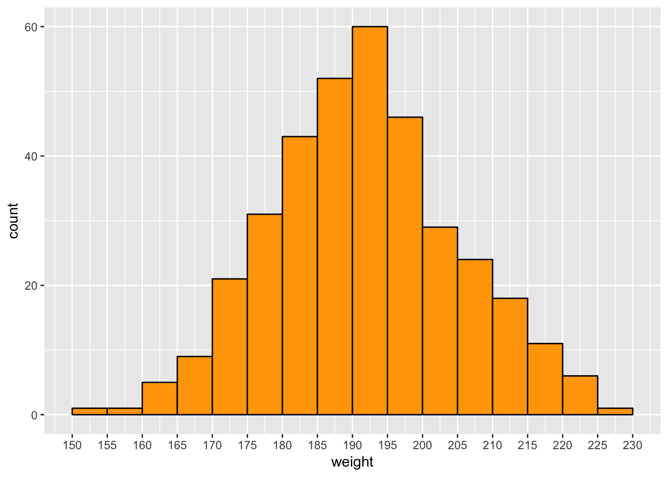
For the women,
regionals %>%
  filter(gender == "Female") %>%
  select(name, weight) %>%
  distinct() %>%
  select(weight) %>%
  summary()
## weight
## Min. :105.0
## 1st Qu.:135.0
## Median :145.0
## Mean :143.7
## 3rd Qu.:150.2
## Max. :220.5
## NA's :2Here the average of 144 lbs is significantly below the average US female weight of 169 lbs (this is probably higher now, the 169 lb average is from data from 2014 or earlier: see here). The weight of 105 lbs. comes from someone listed with a height of 4 ft. 10 in., so I will keep this data point. At the upper end, the 220.5 lbs comes from someone listed with a weight of 100 kg and a height of 5 inches, so I’ll throw this out. The next-lowest weight (195 lbs) seems plausible as it comes with a height of about 6 ft. Here is a histogram of the female weight distribution:
regionals %>%
  filter(gender == "Female", name != "Steph Dekker", !is.na(weight)) %>%
  select(name, weight) %>%
  distinct() %>%
  ggplot(aes(weight)) +
  geom_histogram(breaks = seq(100, 200, 5), color = "black", fill = "orange") +
  scale_x_continuous(breaks = seq(100, 200, 5))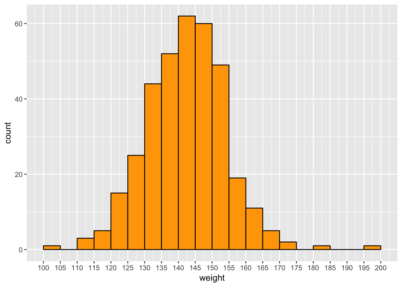
Linda Finish and Bodyweight (Men)
Linda was Event 2 at regionals, so let’s pull out the rows we need. I only need rows with nonzero times, as I used time = 0 to identify people who withdrew from the competition. For people who ran into the timecap of 17 minutes, I used time = -1.
linda_men <- regionals %>%
  filter(gender == "Male", weight != 115, !is.na(weight)) %>%
  filter(event == 2, time != 0)
linda_men %>%
  arrange(rank)
## # A tibble: 353 x 13
## rank_overall id age weight height name event rank points time
## <dbl> <dbl> <dbl> <dbl> <dbl> <chr> <dbl> <dbl> <dbl> <dbl>
## 1 9 105536 29 195 69 Chas… 2 1 100 786.
## 2 1 134617 26 195 69 Sean… 2 1 100 879.
## 3 4 92567 34 229. 72.8 Andr… 2 1 100 729.
## 4 1 153604 28 190 67 Math… 2 1 100 761.
## 5 11 105058 28 220 74 Jona… 2 1 100 744.
## 6 3 697349 30 212. 74.0 Andr… 2 1 100 875.
## 7 2 109346 29 195 69 John… 2 1 100 766.
## 8 12 487949 30 207. 70.9 Moha… 2 1 100 841.
## 9 1 16080 27 192. 69.7 Jame… 2 1 100 746.
## 10 1 158264 28 195 71 Patr… 2 2 94 798.
## # ... with 343 more rows, and 3 more variables: cumulative_points <dbl>,
## # location <chr>, gender <chr>We can look at the fastest overall times (listed in seconds):
linda_men %>%
  filter(time != -1) %>%
  select(name, age, weight, height, time, rank, location) %>%
  arrange(time)
## # A tibble: 183 x 7
## name age weight height time rank location
## <chr> <dbl> <dbl> <dbl> <dbl> <dbl> <chr>
## 1 Andrey Ganin 34 229. 72.8 729. 1 Europe
## 2 Jonathan Gibson 28 220 74 744. 1 West
## 3 James Newbury 27 192. 69.7 746. 1 Pacific
## 4 Mathew Fraser 28 190 67 761. 1 Central
## 5 Adrian Mundwiler 25 183. 67.3 766. 2 Europe
## 6 John Coltey 29 195 69 766. 1 Atlantic
## 7 Roman Khrennikov 23 214. 71.7 771. 3 Europe
## 8 Nicholas Urankar 34 192 70 782. 2 Central
## 9 Gena Malkovskiy 27 216. 70.9 782. 4 Europe
## 10 Chase Smith 29 195 69 786. 1 East
## # ... with 173 more rowsAndrey Ganin in the Europe regional had the fastest overall time of 729 seconds, or 12 minutes and 9 seconds. With a total of 165 reps in this workout, this time corresponds to 1 rep every 4.4 seconds (and there was a lot of walking back and forth between bars)! Europe was a very strong region for this workout - the top 4 finishers in Europe were faster than the first-place finisher in the East.
Here is a plot, along with a linear fit:
linda_men %>%
ggplot(aes(x = weight, y = rank)) +
geom_point(aes(color = location)) +
scale_x_continuous(breaks = seq(150, 230, 10)) +
scale_y_reverse(breaks = c(1:40), minor_breaks = NULL) +
geom_smooth(method = "lm", se = FALSE) +
labs(x = "weight (lbs)", y = "event 2 (Linda) finish")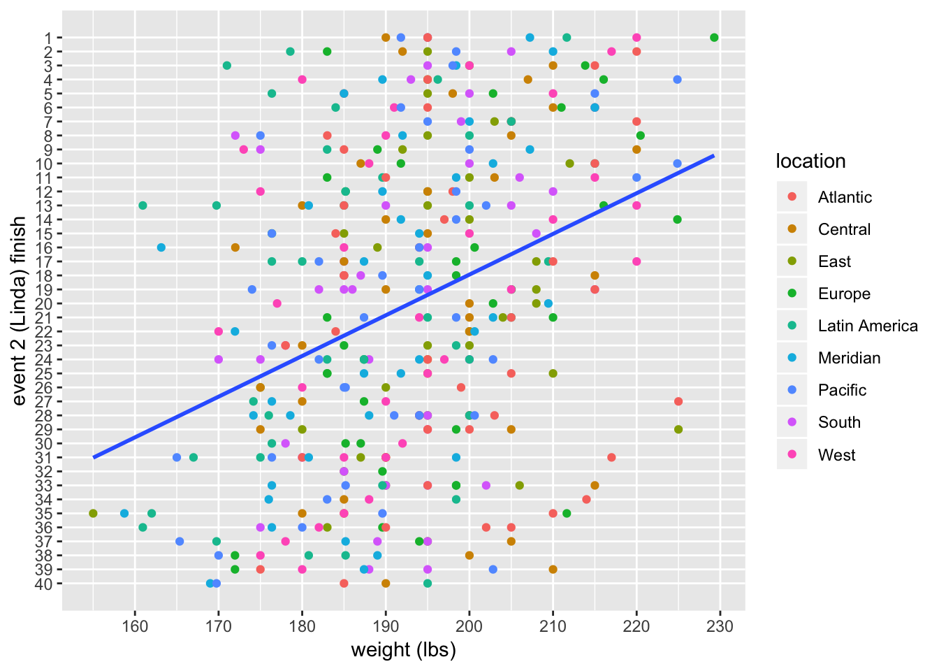 Note: I am treating the rank (finish) as a continuous variable, when it is really a discrete variable.
There does seem to be a relationship between weight and finish, but there is a lot of scatter in the plot. Let’s make things more precise by fitting a linear model.
linda_men_model <- lm(rank ~ weight, data = linda_men)
summary(linda_men_model)
##
## Call:
## lm(formula = rank ~ weight, data = linda_men)
##
## Residuals:
## Min 1Q Median 3Q Max
## -23.3706 -8.9394 -0.2724 8.3181 23.9679
##
## Coefficients:
## Estimate Std. Error t value Pr(>|t|)
## (Intercept) 76.08581 8.02471 9.481 < 2e-16 ***
## weight -0.29073 0.04149 -7.008 1.25e-11 ***
## ---
## Signif. codes: 0 '***' 0.001 '**' 0.01 '*' 0.05 '.' 0.1 ' ' 1
##
## Residual standard error: 10.63 on 351 degrees of freedom
## Multiple R-squared: 0.1227, Adjusted R-squared: 0.1202
## F-statistic: 49.11 on 1 and 351 DF, p-value: 1.246e-11What is this telling us? First, note that the estimated coefficient for weight is negative, but this make sense - higher weight means lower finishing rank. (I flipped the y-axis in the plot above to make it more visually intuitive.) There is a definite association, but the \(R^2\) is fairly low at 12% and the residual standard error is fairly high at 11 places. This makes sense when looking back at the amount of scatter in the plot.
The coefficient of \(-0.29\) for weight means that according to the model, the average finish of men weighing 210 lbs is \(0.29(210 - 180) = 8.7\) places lower than men weighing 180 lbs (lower is better).
Now, there is a problem with using ordinary linear regression here. The outcome variable (event finish or rank) is constrained to be in the interval \([1, 40]\). If we apply the model to weights higher or lower than the weights in the data, we will quickly get meaningless results (finishes \(> 40\) or $ < 1$). This is a good reminder that the linear model is only a model and not a very good one. I would expect that weights higher than around 250-260 lbs. would start to correspond to worse finishes: in other words, there should be an optimal bodyweight for this workout, and weights beyond that would not correspond to better finishes. I also expect the relation to fall off faster than a linear function for weights below 160 lbs.
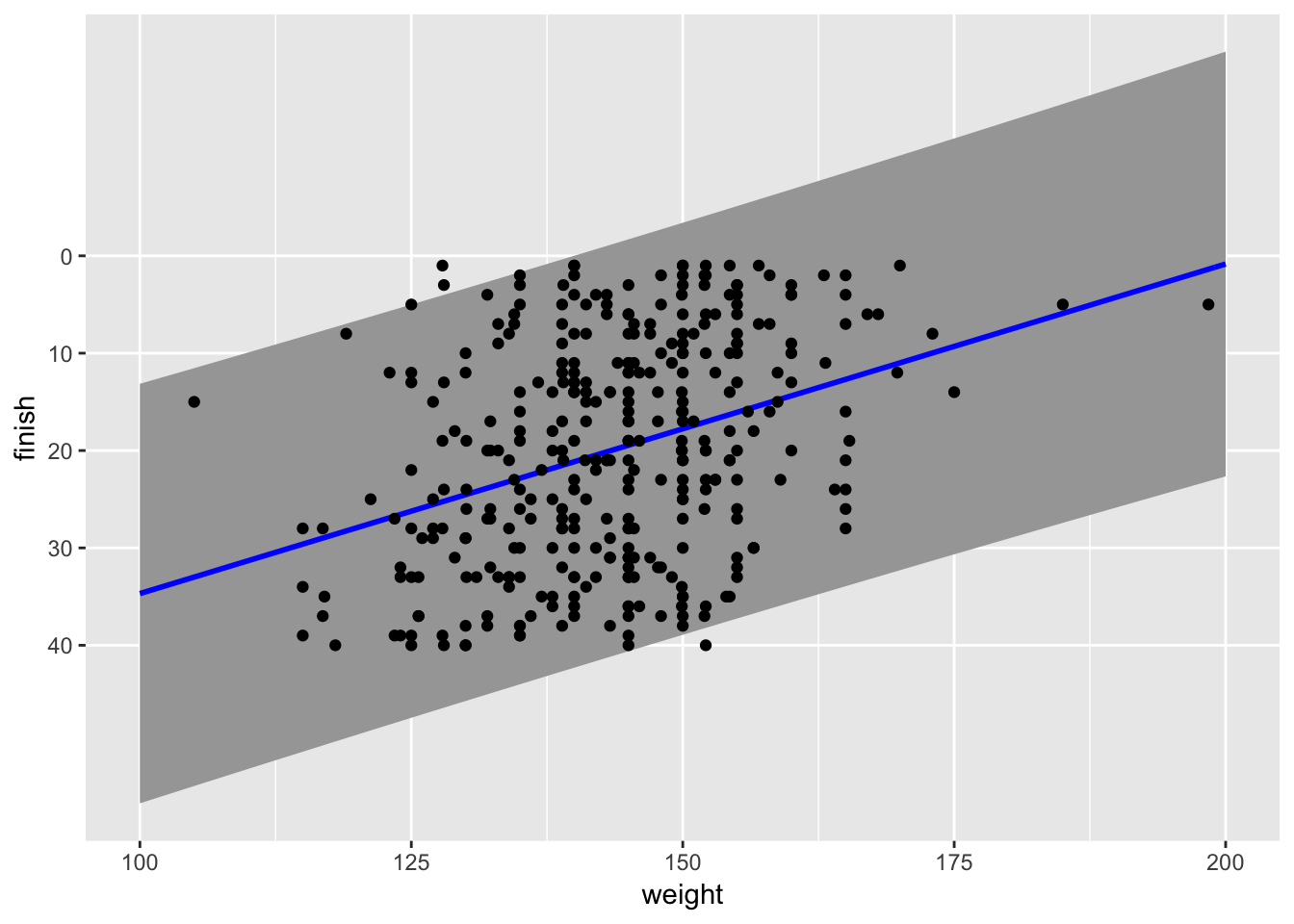
Let’s look at the predictions along with prediction intervals at 95% from the model. This lets us see the large variance in the model.
male_weights = data.frame(weight = c(155:230))
male_predictions <- cbind(male_weights,
                          predict(linda_men_model, male_weights,
                                  interval = "prediction", level = 0.95))
ggplot(male_predictions, aes(x = weight , y = fit)) +
  geom_ribbon(aes(ymin = lwr, ymax = upr), fill = "grey65") +
  geom_line(aes(x = weight, y = fit), color = "blue", size = 1) +
  geom_point(data = linda_men, aes(x = weight, y = rank)) +
  labs(y = "finish") +
  scale_y_reverse(breaks = seq(0, 40, by = 10), minor_breaks = NULL)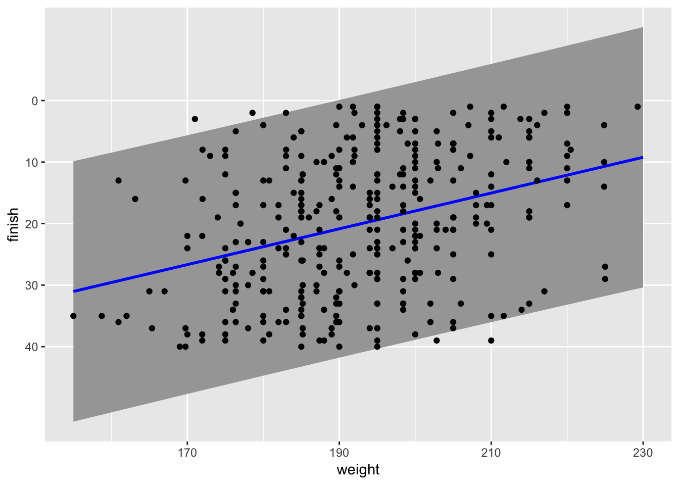
Linda Finish and Bodyweight (Women)
Now for the women,
linda_women <- regionals %>%
  filter(gender == "Female", name != "Steph Dekker", !is.na(weight)) %>%
  filter(event == 2, time != 0)
linda_women %>%
  arrange(rank)
## # A tibble: 353 x 13
## rank_overall id age weight height name event rank points time
## <dbl> <dbl> <dbl> <dbl> <dbl> <chr> <dbl> <dbl> <dbl> <dbl>
## 1 1 55121 25 150 66.5 Katr… 2 1 100 770.
## 2 11 208293 27 140 62 Alex… 2 1 100 990.
## 3 3 8859 25 152. 67.3 Ragn… 2 1 100 783.
## 4 1 168305 23 150 66 Broo… 2 1 100 882.
## 5 1 180250 29 157 67 Emil… 2 1 100 860.
## 6 14 239210 32 170 65.0 Andr… 2 1 100 878.
## 7 1 123582 30 140 63 Cass… 2 1 100 834.
## 8 7 274049 31 154. 65.0 Mani… 2 1 100 947.
## 9 1 163097 24 128. 64.2 Tia-… 2 1 100 844.
## 10 3 103389 30 140 65.0 Caro… 2 2 94 866.
## # ... with 343 more rows, and 3 more variables: cumulative_points <dbl>,
## # location <chr>, gender <chr>The fastest times for the women:
linda_women %>%
  filter(time != -1) %>%
  select(name, age, weight, height, time, rank, location) %>%
  arrange(time)
## # A tibble: 62 x 7
## name age weight height time rank location
## <chr> <dbl> <dbl> <dbl> <dbl> <dbl> <chr>
## 1 Katrin Tanja Davidsdottir 25 150 66.5 770. 1 East
## 2 Ragnheiður Sara Sigmundsdo… 25 152. 67.3 783. 1 Europe
## 3 Cassidy Lance-Mcwherter 30 140 63 834. 1 Atlantic
## 4 Whitney Gelin 33 165 67 834. 2 Atlantic
## 5 Tia-Clair Toomey 24 128. 64.2 844. 1 Pacific
## 6 Emily Abbott 29 157 67 860. 1 West
## 7 Carol-Ann Reason-Thibault 30 140 65.0 866. 2 East
## 8 Andrea Rodriguez 32 170 65.0 878. 1 Latin Ameri…
## 9 Mekenzie Riley 30 155 64 880. 3 Atlantic
## 10 Brooke Wells 23 150 66 882. 1 Central
## # ... with 52 more rowsKatrin Davidsdottir holds the event record, with a time of 12 minutes, 50 seconds. The Atlantic looks like a strong region for this workout: the top 3 Atlantic finishers were faster than the first-place finisher in the Central region.
A plot along with the linear fit:
linda_women %>%
ggplot(aes(x = weight, y = rank)) +
geom_point(aes(color = location)) +
scale_x_continuous(breaks = seq(100, 200, 10)) +
scale_y_reverse(breaks = c(1:40), minor_breaks = NULL) +
geom_smooth(method = "lm", se = FALSE) +
labs(x = "weight (lbs)", y = "event 2 (Linda) finish")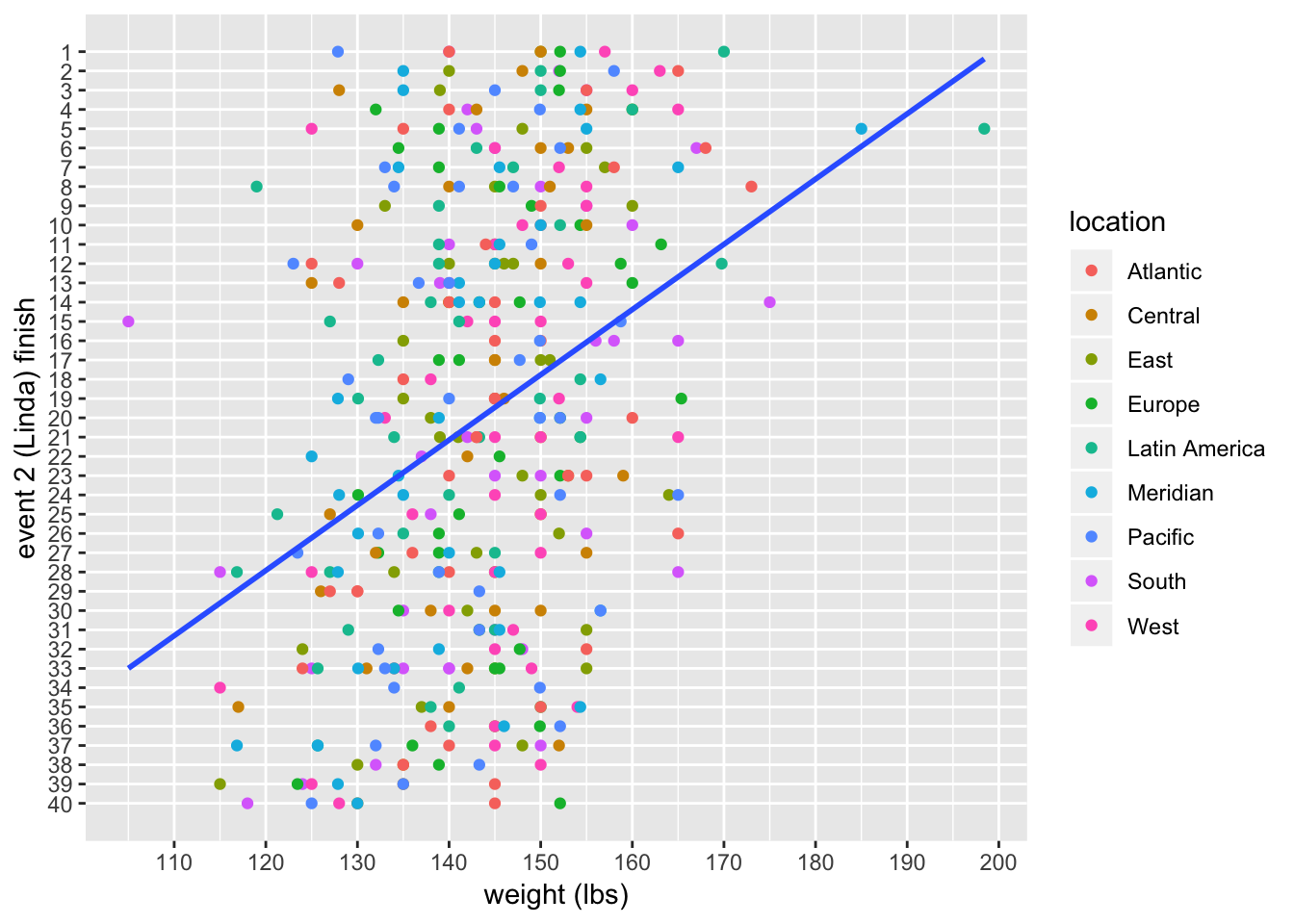 There are more outliers here than there were for the men, but again the overall picture looks like a definite relationship, but one with a lot of scatter. Fitting a linear model:
linda_women_model <- lm(rank ~ weight, data = linda_women)
summary(linda_women_model)
##
## Call:
## lm(formula = rank ~ weight, data = linda_women)
##
## Residuals:
## Min 1Q Median 3Q Max
## -24.2562 -8.4573 0.1888 8.7137 22.9523
##
## Coefficients:
## Estimate Std. Error t value Pr(>|t|)
## (Intercept) 68.53752 6.90259 9.929 < 2e-16 ***
## weight -0.33848 0.04794 -7.060 8.96e-12 ***
## ---
## Signif. codes: 0 '***' 0.001 '**' 0.01 '*' 0.05 '.' 0.1 ' ' 1
##
## Residual standard error: 10.74 on 351 degrees of freedom
## Multiple R-squared: 0.1244, Adjusted R-squared: 0.1219
## F-statistic: 49.85 on 1 and 351 DF, p-value: 8.96e-12The \(R^2\) value and the standard error are almost exactly the same as the model for the men. The coefficent for weight has a larger magnitude: \(-0.34\) for the women comparted to \(-0.29\) for the men. According to the model, the average finish of women at 165 lbs is \(0.34(165-135) = 10.5\) places lower than the average finish of women at 135 lbs (remember that lower is better).
The predictions along with 95% prediction errors:
female_weights = data.frame(weight = c(100:200))
female_predictions <- cbind(female_weights,
                          predict(linda_women_model, female_weights,
                                  interval = "prediction", level = 0.95))
ggplot(female_predictions, aes(x = weight , y = fit)) +
  geom_ribbon(aes(ymin = lwr, ymax = upr), fill = "grey65") +
  geom_line(aes(x = weight, y = fit), color = "blue", size = 1) +
  geom_point(data = linda_women, aes(x = weight, y = rank)) +
  labs(y = "finish") +
  scale_y_reverse(breaks = seq(0, 40, by = 10), minor_breaks = NULL)